How GPUs Communicate: Fundamentals of Distributed Training with PyTorch

The rapid growth in the use of Artificial Intelligence (especially for language modeling tasks) in recent years has been rightly credited to the Transformer architecture. The seminal 2017 paper introduced the concept of self-attention, allowing each token in a sequence to attend to others contextually. This made it possible to build models capable of generating coherent text in an autoregressive manner — that is, using previous tokens to generate the next one. Although autoregression existed before, Transformers made the process scalable and efficient.

A key feature of the architecture, enabling its effectiveness for language modeling, is the ease of parallelizing its operations at different levels. Unlike recurrent neural networks (RNNs) and their derivatives, token-level computation can be parallelized since dependencies are modeled through attention mechanisms rather than sequential states. As a result, training Transformer-based models could be optimized to take advantage of the parallelism offered by GPUs.

One concept observed during neural network training is scaling laws. This refers to the relationship between model performance and its scale, including the number of parameters, the size of the training dataset, and the computational budget. This concept was formalized by Kaplan et al. (2020) and later refined by Hoffmann et al. (2022). While we won’t go into the details in this article, it’s worth noting that larger models have consistently shown better performance.

However, as models grow, it becomes necessary to parallelize the training process, since even the latest-generation GPUs lack sufficient memory to store all parameters, gradients, optimizer states, and activations needed for gradient computation. For this reason, deep learning frameworks like PyTorch rely on libraries that implement communication operations across machines to synchronize parallel computations. These are known as collective operations.

This is the first article in a series that will present the basics of training language models in a distributed setup. In this introduction, we’ll explore the main collective operations used during training and how to use them with PyTorch.

NCCL: The Standard Library for GPU Communication

NCCL (pronounced "nickel") stands for NVIDIA Collective Communication Library. It implements several collectives for GPU-to-GPU and node-to-node communication and is supported by PyTorch. The library is optimized for high bandwidth and low latency communication over PCIe, NVLink (intra-node), and InfiniBand (inter-node).

For instance, in distributed training with data parallelism, each GPU computes gradients locally and, at the end of the forward and backward passes, an all-reduce operation is used to sum the gradients across GPUs. In PyTorch, this is done with torch.distributed.all_reduce, which internally uses NCCL. The sections below will explain how all-reduce works.

Other libraries like MPI and Gloo are also supported by PyTorch. However, while NCCL is recommended for GPU training, Gloo — although GPU-compatible — is inefficient in comparison and should be used primarily for CPU training.

Broadcast: Sharing Data Across GPUs

The broadcast operation sends a tensor from one GPU to all others involved in communication. This way, all GPUs gain access to the same value and can perform consistent computations based on the shared data.

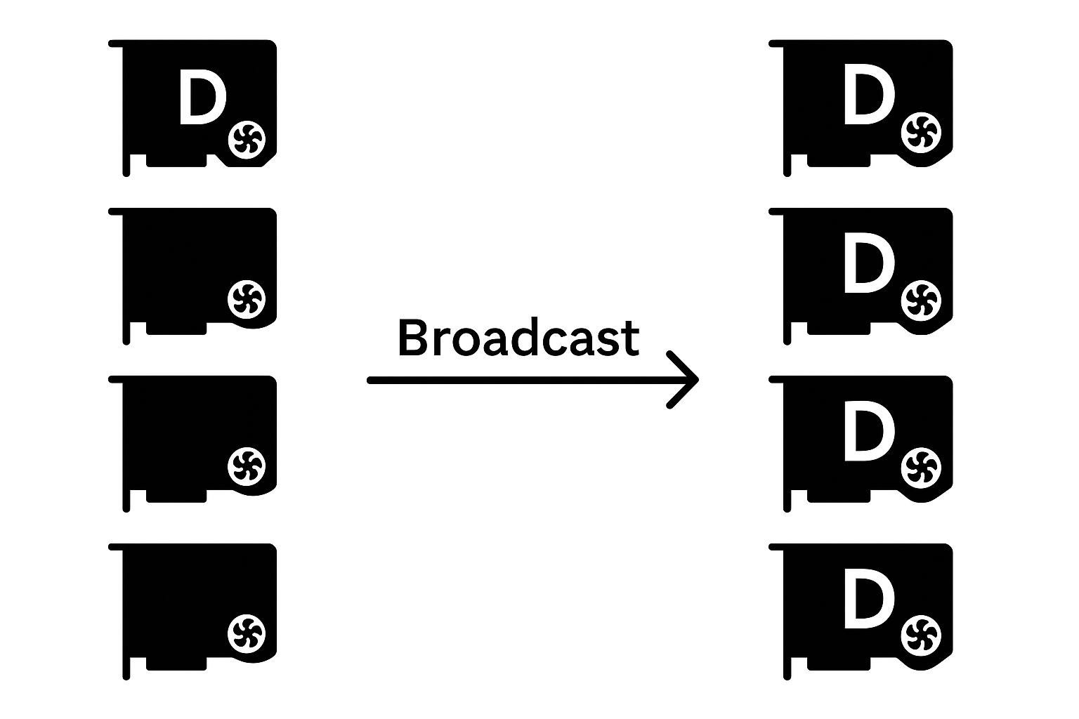
This operation is useful at the start of distributed training when model weights need to be synchronized across replicas. For example, if a single GPU has enough memory to load all weights, they can be loaded onto that GPU, which then broadcasts them to the others, ensuring all replicas start with the same model state.

In PyTorch, the function torch.distributed.broadcast(tensor, src=0) performs this operation, where tensor is the data to propagate and src indicates the source GPU rank.

Reduce and All-Reduce: Aggregating Information Across GPUs

The reduce operation combines distributed information across GPUs using an aggregation function such as sum, mean, or max. The key difference between reduce and all-reduce is the destination of the result: reduce returns the aggregated value only on the root node, whereas all-reduce performs a broadcast of the result to all GPUs.

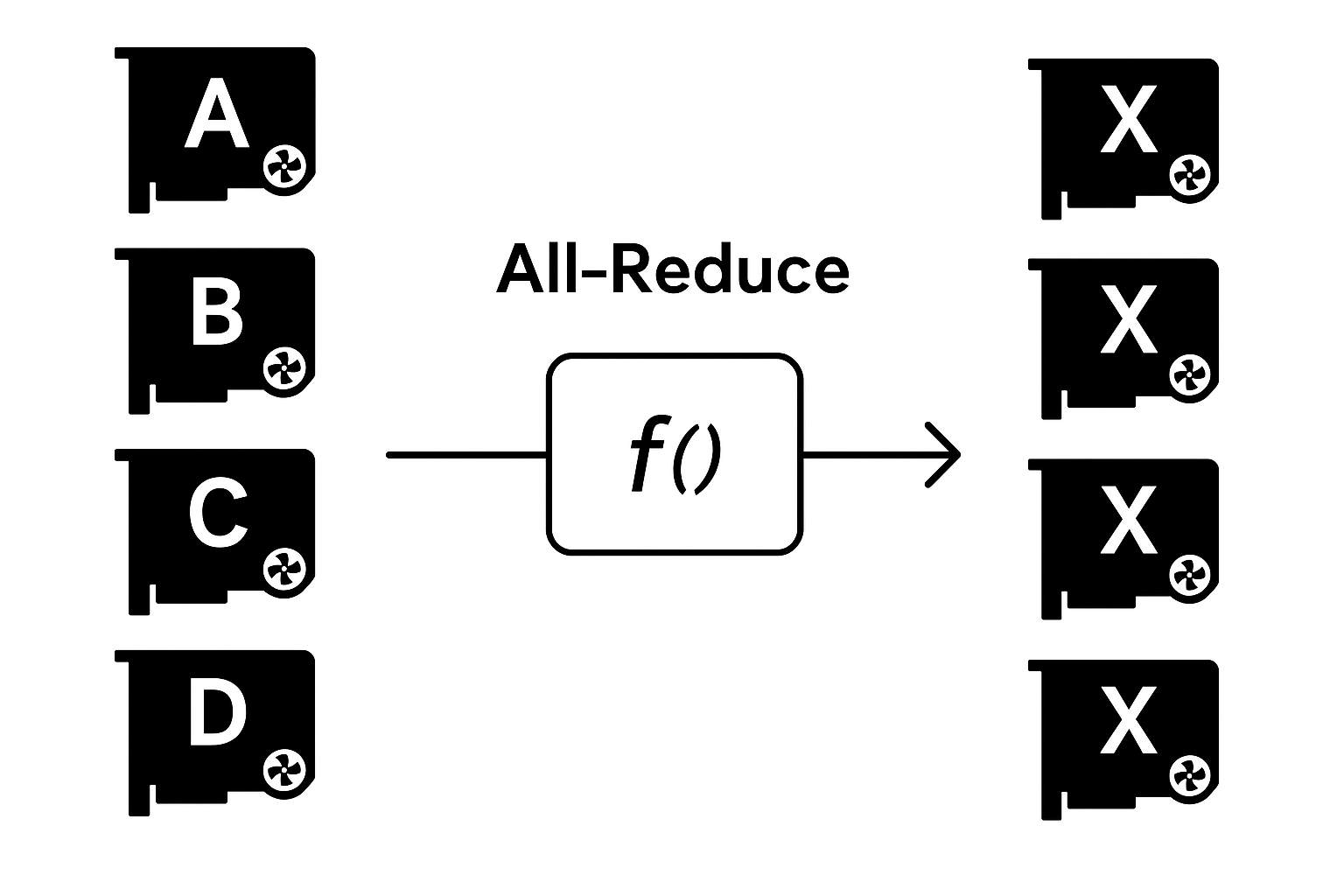
For example, suppose tensor A has values [0, 1, 2] on rank 0 and [3, 4, 5] on rank 1. A reduce operation with sum to rank 0 would result in [3, 5, 7] on rank 0 and leave rank 1 unchanged. In contrast, an all-reduce would result in [3, 5, 7] on both ranks.

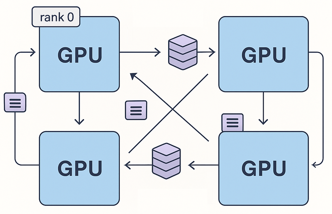
Depending on the communication backend, GPUs can be organized into topologies like rings or trees to optimize aggregation. In a ring structure, for example, each GPU sends its data to the next, which aggregates it and forwards the result until the root node receives the final sum.

A typical use case of all-reduce is in data parallel training: each rank processes a different mini-batch and produces different gradients. To maintain consistency, all gradients must be summed — done via all-reduce. Only after this step can the optimizer update the model weights globally. If all-reduce is skipped, each GPU would apply the optimizer using local gradients, causing model divergence.

The function dist.reduce(tensor, dst=0, op=dist.ReduceOp.SUM) performs a reduce operation in PyTorch, where tensor is the data, dst is the destination rank, and op is the aggregation function.

Gather and All-Gather: Collecting Data From All GPUs

Gather and all-gather operations collect information stored in each GPU. Think of it as a reverse-broadcast where each node has a piece of the data to be collected. To gather all data into a single rank, use gather; to replicate the collection across all GPUs, use all-gather.

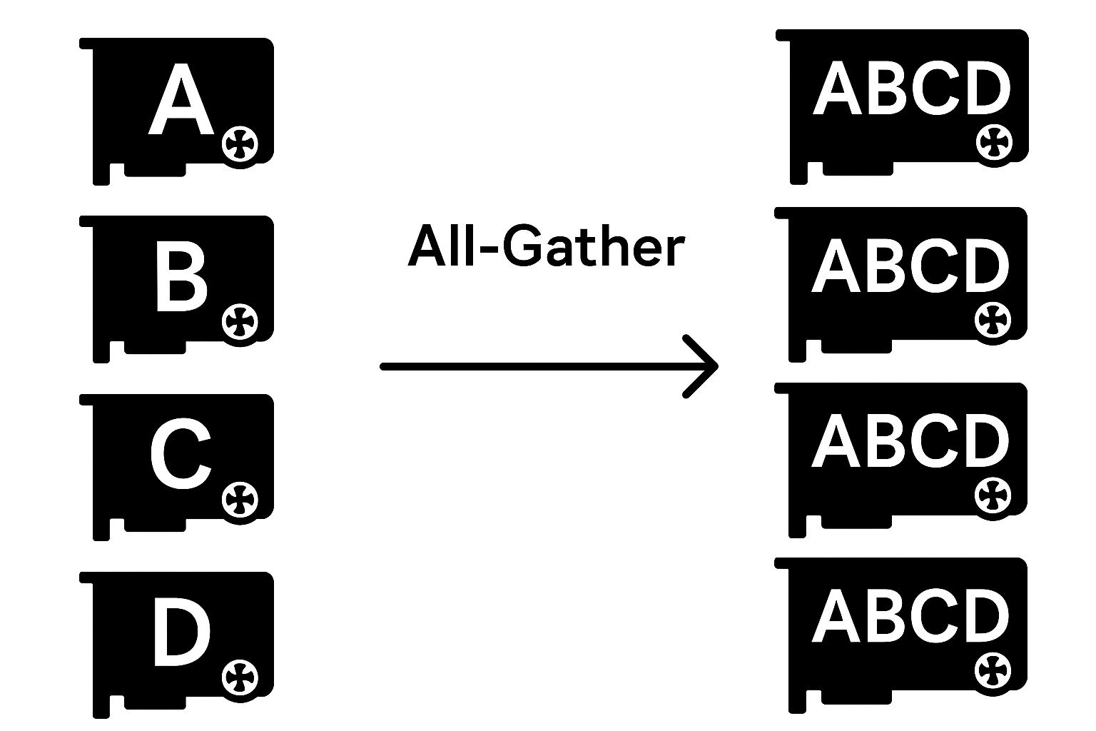
Returning to the earlier example, suppose rank 0 has A = [0, 1, 2] and rank 1 has A = [3, 4, 5]. Before the gather operation, a container (like a list) must be created to hold all tensors. After a gather, rank 0 will have tensor_list = [tensor([0, 1, 2]), tensor([3, 4, 5])], while rank 1 will have None. With all-gather, both ranks will hold the full list.

Note that gather doesn’t alter the original tensor—it merely creates an aggregated view.

All-gather is used in various stages of distributed training. For example, during evaluation, accuracy may be computed on a validation set partitioned across GPUs, and results are gathered into a list to calculate global accuracy.

In a data parallel variation called FSDP (Fully Sharded Data Parallel), model weights, optimizer states, and gradients are split across multiple GPUs (shards). During the forward pass, an all-gather operation collects the necessary weights, which are later discarded from memory. This is handled automatically by PyTorch.

The function dist.gather(tensor, gather_list, dst=0) performs a gather in PyTorch, where tensor is the data, gather_list is the container for collected data, and dst is the destination rank.

Scatter: Distributing Data Slices to GPUs

Scatter is the inverse of gather: when a tensor resides on a single GPU and needs to be partitioned and distributed, scatter is used. You create a list of tensors, one per target GPU.

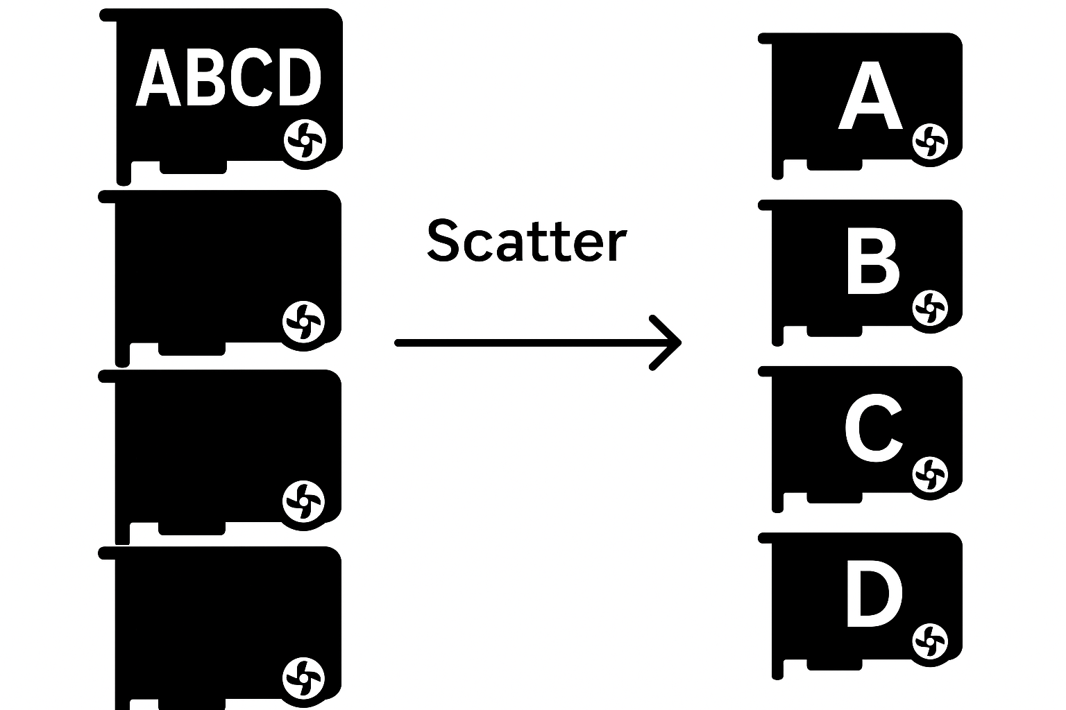
For instance, if rank 0 has tensor_list = [tensor([0, 1, 2]), tensor([3, 4, 5])], a scatter will result in rank 0 having [0, 1, 2] and rank 1 having [3, 4, 5].

The function dist.scatter(tensor, scatter_list, src=0) performs scatter in PyTorch, where tensor is the target tensor on each GPU, scatter_list is the list of data shards on the source, and src is the source rank. Only the source should provide scatter_list; other ranks pass None.

Scatter is rarely used in isolation during training, mainly because it centralizes data on one GPU, which creates a communication bottleneck and contradicts the decentralized training philosophy. However, when combined with reduce, it becomes the widely used reduce-scatter operation.

Reduce-Scatter: Efficient Aggregation With Partitioning

Reduce-scatter applies an aggregation function across GPUs (like reduce) but partitions the result and distributes the pieces (like scatter).

As noted in the all-gather section, in FSDP, weights are gathered and then discarded during the forward pass. During the backward pass, a reduce-scatter operation ensures each GPU receives only its slice of the summed gradients. This reduces memory usage and communication overhead compared to all-reduce.

The function dist.reduce_scatter(output_tensor, input_tensor, op) performs reduce-scatter in PyTorch, where output_tensor receives the distributed results and input_tensor is a concatenated tensor of local shards from each rank, which will be aggregated by op.

Conclusion

This article introduced the main collective operations used in distributed neural network training, particularly for Large Language Models (LLMs). Some operations like barrier (which synchronizes all GPUs) and all-to-all (common in Mixture of Experts—MoE models) were not covered here but are also used in specific contexts. Still, all-reduce, all-gather, and reduce-scatter are the most widely adopted.

In the next articles in this series, we'll explore model parallelism techniques, starting with data parallelism, where the model is replicated across multiple GPUs and each replica performs the forward and backward passes on different data batches.